For data reports: sometimes you want your data ranking in relation to each other visible. And sometimes, you don’t want it visible. Microsoft Excel’s conditional formatting feature allows a quick way to rank data relative to one another visually, using in-cell bar charts, icons and heatmaps. However, for some use case or another, you might want to be able to see the data just the way it is, without the conditional formats. Here’s a quick way to set this up.
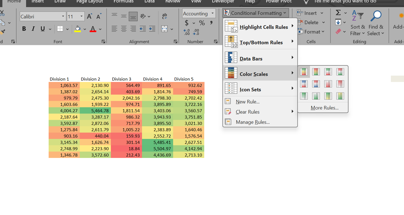
- In your report table, set up the conditional formatting rule as you’d normally do. For this example, the rule I’m using is the “Color Scales: Green-Yellow-Red” rule.
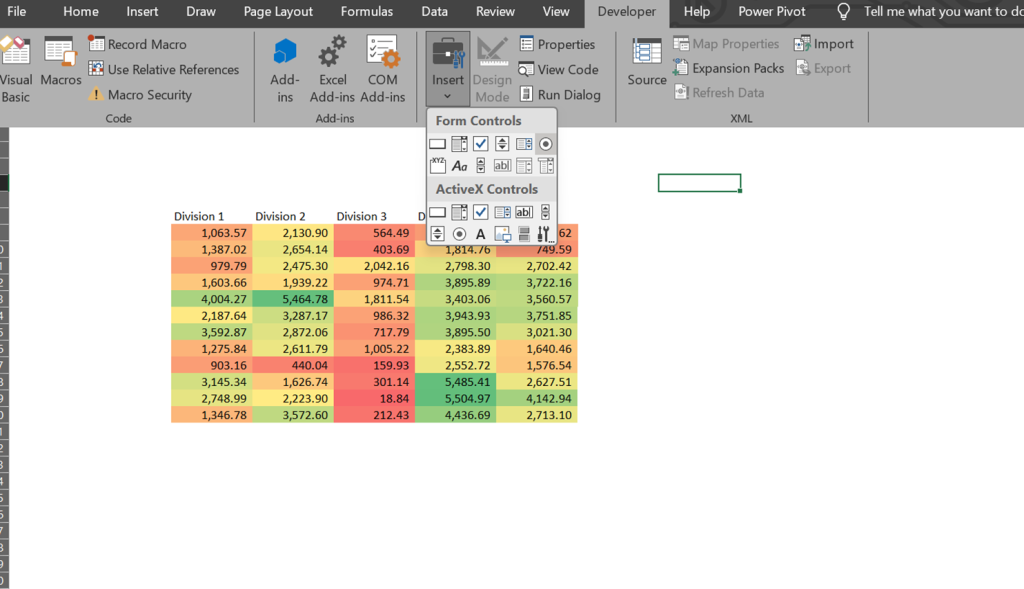
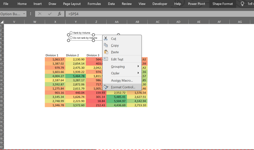
2. Using Form Controls (File > Developer > Form Controls), create 2 radio buttons. Right-click to edit the text and label the radio buttons. One of the radio buttons will be labelled with a “turn on” (or “Rank by volume” in my instance), and the other will be labelled with a “turn off” – “Do not rank by volume”.
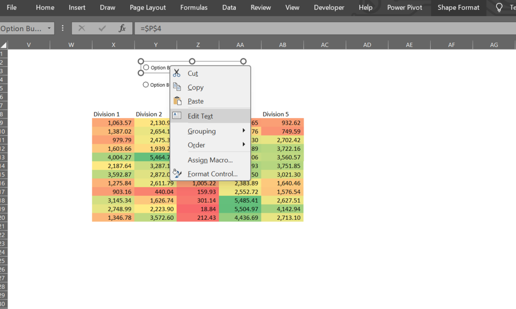
3. Right-click on each of the radio buttons and go to “Format Control”. Set up the cell link – I’ve used cell $X$2 for my example.
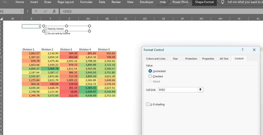
Ensure that you use the same cell link for both radio buttons i.e. both radio buttons must refer to the same cell – $X$2 in my instance.
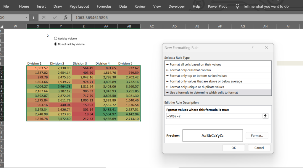
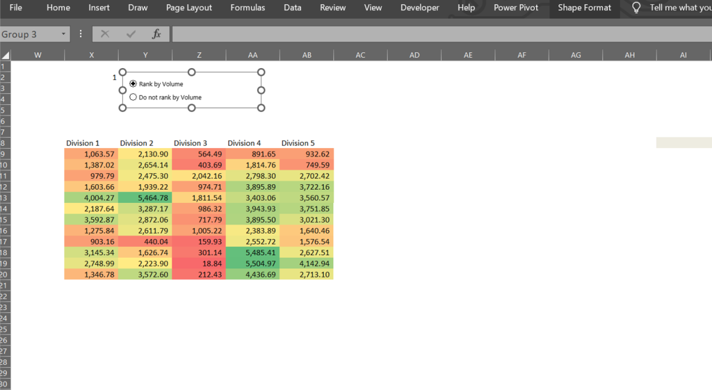
When this is set up well, it will look like the below – on clicking the “Rank by volume” radio button, $X$2 will have the value 1 and on clicking the “Do not rank by volume” radio button, $X$2 will have the value 2 (it may be the other way round depending on which button you set up first, but each radio button should yield a different output in $X$2 when clicked)
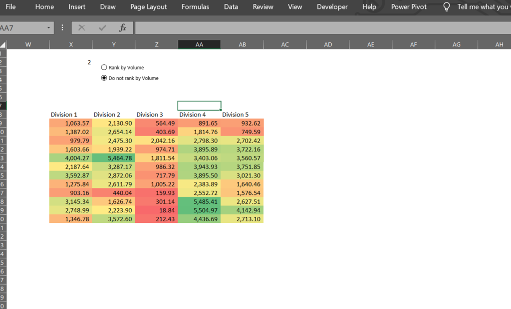
4. Finally, go to Conditional Formatting and set up a formula-based rule: to format values where “=$X$2=2” with white fill color and black font color