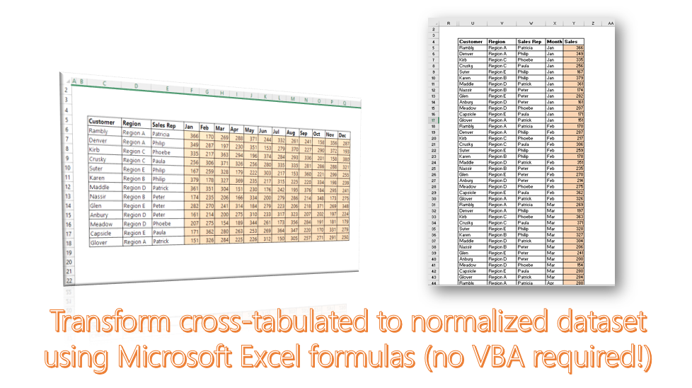
When working with tables of data, the table set up usually encountered is the cross-tabulated or matrix data format. However, this dataset is not optimized for further analytics in Business Intelligence software like Tableau or Power BI. These software require datasets to be set up in a manner that ensures that a row represents a record.

Converting a cross-tabulated data set (also known as unpivoting or reverse pivoting) data in Microsoft Excel can be a daunting task when attempted manually. If, for instance like the data set above, your data set contains sales records for 13 customers for 12 months in a year, you would need to recreate 156 rows of data.

Reverse pivoting can be performed with Power Query’s Get and Transform Data, and JavaScript code on Google Sheets. But if you do not have Power Query installed and don’t want to dabble into programming, there is a formula-based approach for performing this reverse pivot operation in Microsoft Excel. You can get this done within minutes, even if your data runs into thousands of rows and columns.

Step 1: Number the items in the row and the column, starting from the first item (item, not header, should be 1)

Step 2: We are now going to designate three cells. One to hold the total count of rows (A), the second the total count of columns (B), and the last as a check, which will hold the product of both totals (C). The MAX() function will be used to get the value in (A) and (B). We are also going to dedicate two columns as helper columns – one for the rows (D) and the other for the columns (E).

Step 3: Set up the column headers for the normalized data set. This will include the dimensions of the data (Customer, Region and Sales Rep in my example) and the measure (Month in my example). For my example, these are 4 columns, but might be more if there were more dimensions. The column headers should be set up right next to the look up columns (E in the set up above)

Step 4: So we understand the normalized data set must have 156 rows (as designated cell C above denotes). 156 records because each of our 13 customers will have 12 records, one for each month in the year per the data set. We will then need to number these 156 rows in preparation for the normalized data set that will be brought in using =VLOOKUP and =HLOOKUP operations. This numbered set up will be done in the lookup columns and will go by the logic above – 1 row for each customer, 12 times. This is what it looks like:

Typically, this numbering does not follow any of the Excel autofill styles and has to be manually generated. But there’s a formula to help out. Simply enter 1 on the first row of the row and column lookup columns, and enter the following formulas from the second row and drag downwards to cover 155 (156 minus the first row) rows.

Formula for 2nd row of COLUMN LOOKUP:

=IF(S5=$U$1,T5+1,IF(S6<=$U$1,T5,0))

Formula for 2nd row of ROW LOOKUP:

=IF(S5<$U$2,S5+1,1)

Step 5: Now we have our 156 record rows numbered, we can go ahead to set up our =VLOOKUP and =HLOOKUP formulas to convert the cross-tabulated data to a normalized form.

To make the formula breakdown easy to follow along, I have created two named ranges on the initial cross-tabulated dataset. One for the full data (“FullDataSet”), and the second for the columns and their numbering (“ColumnHeaders”). Named Ranges can be created by accessing the Formula tab on the ribbon and clicking Name Manager (or by using the keyboard shortcut Ctrl+F3, or simply selecting the range to be named and typing the name directly into the Name Box (box to the left of the formula bar on the Excel user interface).

I have also brought in the column number of the dimensions of the dataset, these will serve as references for the column index part of the VLOOKUP formulas and make setting up those formulas easier.

As mentioned, a combination of VLOOKUP and HLOOKUP formulas will be used to bring in the data. HLOOKUP will be used to bring in the dimension currently set up as columns (Months in the example), while VLOOKUP will be used to bring in all other dimensions and the measure.

The formulas will be set up as follows:

The formulas used by column are below (row 1 formulas are referenced):

Customer: =VLOOKUP($S5,FullDataSet,U$3,FALSE)

Region: =VLOOKUP($S5,FullDataSet,V$3,FALSE)

Sales rep: =VLOOKUP($S5,FullDataSet,W$3,FALSE)

Month: =HLOOKUP($T5,ColumnHeaders,2,FALSE)

Sales: =VLOOKUP($S5,FullDataSet,Y$3+$T5,FALSE)

You would notice I stepped into the formula will creating them to add dollar signs ($) in front of the references to convert them from relative to mixed references. This makes it easy to drag out the formulas and have them still work correctly, which removes the work of retyping formulas one line after the other. The logic of the mixed referencing is below

$S5 – locks formula to column S (Row lookup column) and ensures every time I drag out the formula to other cells it retains it referencing to column S. No dollar sign in front of 5, which allows the formula to increment when dragged to other rows (as $S6, $S7, $S8, etc)

U$3 – locks formula to row 3 (column index rows) and ensures everytime I drag out the formula to other cells it retains it referencing to row 3. No dollar sign in front of U, which allows the formula to increment when dragged to other columns (as V$3, W$3, etc)

The data has successfully been transformed from matrix to normalized data set.