A dynamic calendar in Excel is set up to present the calendar for a selected month and year and automatically updates when the month and year are changed.

There are preset Excel templates containing dynamic calendars that are accessible to all Excel users from the File>New options. These have been created with complex array formulas and are ready to use. However, if you need to create a calendar for specific dashboard applications and need one with formulas you can easily alter and work with, this tutorial is for you.

Step 1: On a new worksheet, designate input cells for the year and month, and name them.

For my example, I’m using cell A3 for the year and A4 for the month. I have named both cells CurrYear and CurrMonth respectively.

Step 2: Create the calendar header row, with the weekday names. Add a helper row for the weekday numbers.

This was done by inputting the weekday names on a new row and formatting these cells to resemble headers (solid fill with white borders for my example)

Step 3: Determine the weekday number of the first day of that month

Here, we are going to utilize two Excel functions: =DATE() and =WEEKDAY()

The DATE function returns the current date when provided arguments for the year, month and day.

The WEEKDAY function returns a number representing the day of the week when provided a serial number for the date and a return type (week order). It can work with different week orders – Sunday to Saturday, Monday to Sunday, etc. But since the calendar we are building starts from Sunday, we will use the default order or order (1) – Sunday to Saturday

Back to our example: I determined the weekday number for the first day of the focus month by using the formula below: the answer was 6.

=WEEKDAY(DATE(CurrYear,CurrMonth,1))

Step 4: Create a formula logic that deducts the difference from the weekday from 1 if it is more than 1, and returns it if it is 1

This formula will be a condition-based logic using the =IF function. This is what it looks like:

=IF(WEEKDAY(DATE(CurrYear,CurrMonth,1))=1,DATE(CurrYear,CurrMonth,1),DATE(CurrYear,CurrMonth,1)-(WEEKDAY(DATE(CurrYear,CurrMonth,1))-1))

Place this formula in the first cell of your calendar as shown below:

Next, increment this number by 1 (e.g formula in cell D6 above will be =C6+1), and drag it out to the entire first row of the calendar, as shown below.

On the next row, create a formula that adds 7 to the cell above, and drag this out to the rest of the row and 3 more rows below:

Step 5: Format the calendar cells as “dd” in custom number format

Select all the cells in the calendar table range, open up the Format Cell dialog (select “Format Cell” in the dropdown that comes up on right-click, or use the keyboard shortcut Ctrl+1), go to ‘Custom’ in the number format category, and enter ‘dd’ in the ‘Type’ input box

This action will change the date numbers from serial numbers to normal-looking dates.

Step 5: Use conditional formatting to highlight the dates in the month in the calendar range

First, change the font color of the dates to grey, then select the range, go to Conditional Formatting options and select New Formatting rule. Type in the formula below in the input box, and click Format to select black as the font color.

=$A$4=MONTH(C6)

[Note: $A$4 is the reference to the currMonth range, adjust as applies to your worksheet.

While setting up the New Formatting Rule, ensure C6 (reference for the beginning of the calendar range) is reflected as a relative cell reference with no dollar signs – i.e. not as a mixed ($C6 or C$6) or absolute ($C$6) reference. This will ensure the conditional formatting rule will apply to all cells and not just the first cell in the range]

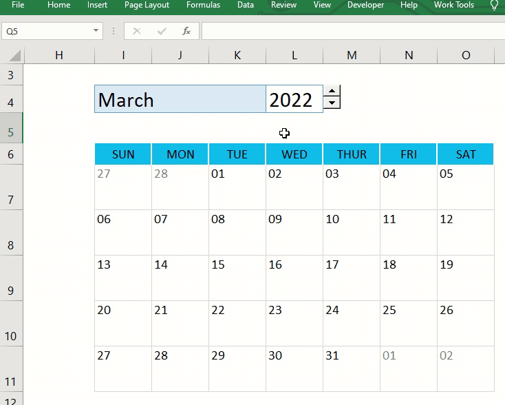
Your calendar is set up for use. And it is dynamic: when you change the year or the month or both, the calendar updates itself to match the new settings.

You can choose to create data validation or dropdown UI to ease the process of updating the year and month as shown below: