If you have ever needed to perform a lookup function and encountered Not Available (#N/A) errors due to wrong name ordering, you are going to love this hack.

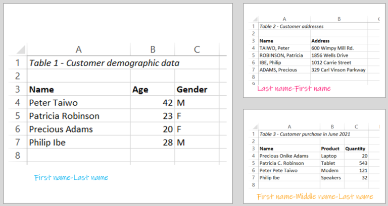
The wrong name order issue comes up commonly when working with human names – employee names or customer names – in Excel. Data analysts face this when trying to consolidate data from users that are not decided on whether to use First Name-Last Name or Last Name-First Name convention. Here’s what this looks like:

So how do you get all names into a unified order, so you can conduct your lookup analysis seamlessly? Through a combination of 5 TEXT Excel functions (namely =LEFT, =RIGHT, =MID, =FIND and =LEN).

The steps to take are as follows:

1. First, decide the name order convention you want to use as the standard, and determine the degree of deviation of each dataset from that standard. For my example, I am making the First Name-Last Name convention the standard. I have noted what will need to change on each table to ensure adherence to this standard.

2. On each table that is deviated from the standard (Tables 2 and 3 in this example), you will need to extract the names using the TEXT functions above.

Before we get into the extraction task proper, here are the TEXT functions we will use and what they do:

• LEFT() – extracts a specified number of characters from the text in a cell starting from the leftmost part of the cell. The argument for this function is:

=LEFT([text containing characters to be extracted],[number of characters to be extracted])

• RIGHT() – extracts a specified number of characters from the text in a cell starting from the rightmost part of the cell. The argument for this function is:

=RIGHT([text containing characters to be extracted],[number of characters to be extracted])

• MID() – extracts a specified number of characters from the text in a cell, starting from a specified point. The argument for this function is:

=MID([text containing characters to be extracted],[position of the first character to be extracted],[number of characters to be extracted])

• LEN() – returns the total number of characters in a cell. This will come in useful when trying to establish the starting point of an extraction – more on this shortly. The argument for this function is:

=LEN([text containing characters to be counted])

• FIND() – looks within a text in a cell and finds a specified character or text string. We will use this formula to establish where the space bar is within a string, which will help in determining the bounds for the extraction task. The argument for this function is:

=FIND([character or string to be searched for],[text containing the character/string being searched for],[starting point for the search within the text; 1 if omitted])

Putting what we now know about the 5 TEXT functions together, here’s what we can now do:

• extract the first word in a cell (with =LEFT), using FIND() to determine the number of characters to be extracted from the position of the space (” “) character separating the first word from the others

• extract the last word in a cell (with =RIGHT); number of characters to be extracted will be the difference between the total number of characters in the cell (with =LEN) and the position of the space (” “) character separating the last word from the others (with =FIND; 3rd argument – starting point of search – will be determined by the total number of words in the cell)

3. As we want the final order to be First Name-Last Name, we will use two helper columns – the first to extract the first name from the original name column, and the second to extract the last names – in each of the two tables requiring transformation.

4. Now to the magic. Insert the TEXT formulas that will extract the first and last words in each table.

For the first table, this is pretty straightforward: use the formulas defined above, taking note to remove two extra characters instead of just one while extracting the first word (because of the comma in between the two words):

For the second table, the same logic applies, but a slight twist: because there are 3 words (first-name, middle-name, last-name) instead of 2 words (first-name, last-name) we have encountered so far, we will need to apply 2 FIND functions: the first to find the space separating the first two words, and the second to use the output of the first FIND as the starting point for the search.

5. Now the first and last names have been extracted, the last step is to merge the names back together so they are maintained in one column. You can do this with =TEXTJOIN function (for newer versions), CONCAT function, or simply using the ampersand sign. Snapshots using the last two results are below.

While merging, you can decide to clean out extra spaces if you believe there are any (I show how to do this in this hack) or transform the text to proper case for a uniform feel.

Once you are satisfied with the corrected names, you can copy them, and paste as values over the original name column, and you are all done!

It must be added that this hack only works seamlessly based on the following assumptions:

• names are separated from one other with a space

• name structure is uniform on each table. If, say Table 2 had a mixture of Last name-First name and First name-Last name records, some preliminary work will need to be done to sort out those orders before the steps above can be executed.