Have you come across a scroll bar that makes an Excel chart dynamic, like shown below:

This scroll bar is a form control that has been programmed to increment on click, and this action automatically adjusts the range of the chart in view. The chart data is made dynamic by the use of the OFFSET function, a lesser known but very effective function in Excel.
This set up is usually used to optimize viewing areas on Excel dashboards and get in more data than can be traditionally fit in. It also helps to keep dashboards clutter-free and clean by enabling the user to focus on only a particular set of data at a time.
This tutorial will show you how to set one up.
First step is to set up the data to be presented in a tabular form as shown below (just like you would set up any normal data for charting).

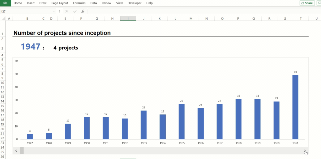
This data set has 74 records, representing the number of years from 1974 to 2020, and number of projects per year.
Next, create a horizontal scroll bar by going to the Developer tab, and inserting a scroll bar form control. Draw out the shape you desire (drag your cursor to the right for a horizontal scroll bar, and drag it downwards for a vertical scroll bar)

Now program the scrollbar. Right-click your scroll bar to bring up the dialog box below and click ‘Format Control…’

… and set up the cell link to a designated cell (I’m using cell $G$1 for this demonstration)

Since this dataset has 74 records, I make 75 the maximum value to avoid endless scrolling that will exceed the range of the data.
The incremental change has been left as 1 for this example. You could change it to adjust the number of views (for instance, I could make it 15 so that the chart will have only 5 views (75/15)).
Once the scroll bar has been programmed, you can test it out. It should work as shown below (incrementing the value in $G$1 by one step with each click of the right arrow on the scroll bar, and reducing the same value by one with each click of the left arrow):

Next: set up the dynamic chart data. I want my dynamic chart to show 15 records at a time, so I’ve designated a new table area on the same sheet with 15 rows that will contain the =OFFSET function

Next step is to input the =OFFSET function that will be extended into all 15 rows. The formula is as follows:
=OFFSET(B2,$G$1,0)

Extend this formula into the remaining 14 rows and the next column.

If your scroll bar cell link ($G$1) is at 1, it will not look like much has happened as the dynamic chart will mirror the first 15 records of your original data set. But when you update the cell link value by clicking the right arrow of the horizontal scroll bar, you will notice the values changing.
The OFFSET function works by returning the value in the cell representative of the row and column displacement from the reference cell.

The above OFFSET formula is set up to ensure the row displacement from the reference cell (which is always the row above the data) updates when the scroll bar (which updates the cell link on change) changes.
Next, create a bar chart using the data in the dynamic chart range.

And this is how the chart should work: