You might have come across the above feature in Excel – a cell with a drop-down list – and wondered how it was set up. This tutorial will show you how to create a drop-down list in MS Excel.

Step 1: Create the list that you want to show up in the drop-down in a table/range of Excel rows. In this example, I have set up the list – names of states in Nigeria – in rows B86:B122

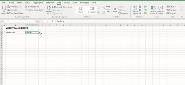
Step 2: Select the cell you want to set up the drop-down menu in – this is cell C3 in my example – and select “Data Validation” (Data – Data Tools – Data Validation)

Step 3: In the dialog that comes up, change “Any value” to “List”, and click into the Source field, and highlight the range of the list you want to show in the drop-down (range B86:B122 in my example).

And the list is all set up!

You can update the range of the list by adjusting the range referenced in the Source field from the Data Validation dialog box.