Between the tasks of cleaning data and generating data reports, is the data query phase. During this phase, efforts are made to make meaning of the data at hand, to get answers to precise questions within a database that has thousands of rows and columns. This squad of Excel functions is here to help you execute data query tasks with ease.

The Data Query Function Squad

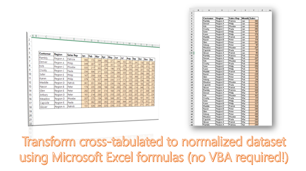
Imagine you had a dataset like the one below:

If you wanted to answer questions about the sales performance across the two dimensions of time (months) and products [produce items] without visually referencing the table, the following functions can come in handy.

• VLOOKUP() – Looks for a value in the leftmost column of a table, and then returns a value in the same row from a column that you specify. Can help answer questions like “How many Carrots did we sell in March, by referring to ‘Carrots’ – which is in the leftmost column of the table, the whole table range, the column number in the table ‘March’ is in, and indicating how precise the match should be (FALSE means perfect match). The syntax for the =VLOOKUP function for the query above is below:

=VLOOKUP (“Carrots”, A1:H11, 4, FALSE)

• INDEX() – Returns a value or reference of the cell at the intersection of a particular row and column, in a given range. INDEX() is perfect when you know the table, the row number in the table, and the column number in the table, of the cell whose value you need.

And even when you do not know the exact row and column number, you can pair INDEX with other functions to get your result. More on that below. You can use INDEX to answer a range of questions from the simple to the complex – one of the simpler ones (“What is the 4th product on the product list?” is in the snapshot below:

• MATCH() – Returns the relative position of an item in an array that matches a specified value in a specified order. So MATCH will give you the 4th item, the 3rd item, the 6th item in any list once you provide the range of the list, and the position number you are looking for. The key phrase in working with MATCH() is “relative position” – notice how the return for the two functions below differ because of a slight change in the referenced range (first range starts from M7, the second starts from M8).

See =MATCH() in action below in our reference data set:

What’s exciting about MATCH() is that it can be paired with =INDEX() to perform a lookup when the row number or column number to complete the =INDEX() function is not known, but the name of the header is known. See the INDEX-MATCH in action below:

• HLOOKUP() – Looks for a value in the top row of a table or array of values and returns the value in the same column from a row that you specify. Can help answer questions like “How many Carrots did we sell in March, by referring to ‘March’ – which is in the topmost row of the table, the whole table range, the row number in the table ‘Carrot’ is in (we use =MATCH to derive this, the mechanics for this function is described above), and indicating how precise the match should be (FALSE means perfect match). The syntax for the =HLOOKUP function for the query above is below:

=HLOOKUP(“March”,A1:H11,MATCH(“Carrots”,A1:A11,0),FALSE)

• MAX() – Returns the largest value in a set of values. Can help answer questions like “What was the highest monthly sales reported for [product/time]?” In the example below (highest monthly sales for Tomatoes), the syntax for the =MAX function is below:

=MAX(B10:G10)

• MIN() – Returns the smallest value in a set of values. Can help answer questions like “What was the lowest monthly sales reported for [product/time]?” In the example below (lowest overall monthly sales), the syntax for the =MIN function is below:

=MIN(H2:H11)

LARGE() – Returns the n-th largest value in a data set. For example, the fifth-largest number. Can help answer questions like “What was the 2nd highest overall sales reported?” with the formula below:

=LARGE(H2:H11,2)

For data query tasks, you can pair =LARGE with INDEX-MATCH lookups to respond to queries like “In what month did Green beans record the 3rd highest sales?” as shown below:

• SMALL() – Returns the n-th smallest value in a data set. For example, the fifth-smallest number. The syntax is similar to that of =LARGE, and just like the example with =LARGE above, =SMALL’s power in data query tasks is when paired with lookup functions (like INDEX-MATCH) to answer questions like “What product had the 3rd lowest sales for the month of May?” as shown below:

ADDRESS() – Creates a cell reference as text, given specified row and column numbers. ADDRESS can be used as shown in the snapshot below:

INDIRECT() – Returns the reference specified by a text string. There are several uses of the =INDIRECT function (click here to see 5 ways), but for this data query post, we are going to focus on the ability to convert the cell address returned by the =ADDRESS function into the actual cell value. In the rare instance where you know the row number and column number of the cell value you are looking for, but are not sure of (or might not need) the table range, you can pair the =ADDRESS and =INDIRECT to create a lookup formula as shown below. This has a dual function as an error check/data validation system, to for instance confirm if a time series data has been entered in the same position across all worksheets in view.