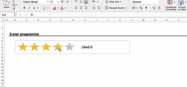
Here is a 5-star ranking system I set up in MS Excel, using minimal VBA code. It really takes just 5 steps to set up, and can be up and running in minutes.

Step 1: Open a fresh worksheet in MS Excel, and create five 5-point star shapes and a text box. Ensure all five 5-point stars are the same size (best to create one and replicate it four times) and are on the same row, distributed horizontally.

Step 2: Name each shape, using the name box. Each shape must end with the number the star corresponds to. For instance, I used Star1, Star2, Star3, Star4 and Star5. Also, name the text box – I used the name ‘StarMeaning’ for the text box

Step 3: Designate two cells on the worksheet – one to receive the name of the selected shape, and another to extract the last character in the name string (with a formula that uses the Excel functions =RIGHT() and =VALUE(): =RIGHT() extracts the reference number of characters in a string from the right as string, =VALUE() converts the output string from the RIGHT() function into a value).

I have set these up and named them ‘SelShape’ and ‘SelNum’ respectively.

NB: When you are setting up there will be nothing in SelNum and SelShape: the values seen in the above snapshots are because this is a walkthrough on an already programmed worksheet

Step 4: Set up the VBA macro. Access the Visual Basic Editor from the Developer Tab and click Insert >> New Module to open a new module, and enter the below code. The explanation for each part of the code is included in the lines beginning with ”

Sub Star_Select()
  
 ''STEP 1 - GET THE NAME OF THE SELECTED SHAPE (STAR1, STAR2, ETC)
 
 ShapeName = ActiveSheet.Shapes(Application.Caller).Name
 
 ''STEP 2 - WRITE THE NAME OF THE SELECTED SHAPE TO A NAMED RANGE SET UP IN THE WORKSHEET CALLED SELSHAPE.
 ''ANOTHER NAMED RANGE ON THE WORKSHEET (SELNUM) EXTRACTS THE ENDING NUMBER ON THE SHAPE NAME USING THE RIGHT() FUNCTION
 
Range("SelShape").Value = ShapeName
 
 ''STEP 3 - USING THE NUMBER EXTRACTED INTO THE NAMED RANGE SELNUM, CHANGE THE FILL COLOR TO YELLOW, FOR ALL SHAPES NAMED /STAR#/ (# BEING ALL NUMBERS UP TO THE SELECTED SHAPE NUMBER)
 
 For i = 1 To Range("SelNum").Value
 
    With ActiveSheet.Shapes.Range(Array("Star" & i))
        .Fill.ForeColor.RGB = RGB(255, 192, 0)
    End With
 
 Next i
 
 ''STEP 4 - IDENTIFY IF THERE ARE ANY STAR SHAPES NAMED WITH NUMBERS GREATER THAN THE SELECTED SHAPE (UP TO 5)...
 
LastNum = 5 - Range("SelNum").Value
  
 If LastNum = 5 Then
 Exit Sub
 
 ''STEP 5 - ...AND IF THERE ARE, CHANGE THEIR FILL COLOR TO GREY
 
 Else

     For j = Range("SelNum").Value + 1 To 5
    
        With ActiveSheet.Shapes.Range(Array("Star" & j))
            .Fill.ForeColor.RGB = RGB(200, 200, 200)
        End With
  
    Next j
  
  End If
  
''STEP 6 - BRING IN THE DESCRIPTION OF THE MEANING OF THE SELECTED STAR, BASED ON THE NUMBER IN THE SELECTED SHAPE NAME

Dim aLabel As Shape
Set aLabel = ActiveSheet.Shapes("StarMeaning")

Select Case Range("SelNum").Value

    Case Is = 5
        aLabel.TextFrame2.TextRange.Characters.Text = "Loved it"
    Case Is = 4
        aLabel.TextFrame2.TextRange.Characters.Text = "Liked it"
    Case Is = 3
        aLabel.TextFrame2.TextRange.Characters.Text = "It was okay"
    Case Is = 2
        aLabel.TextFrame2.TextRange.Characters.Text = "Disliked it"
    Case Is = 1
        aLabel.TextFrame2.TextRange.Characters.Text = "Hated it"

End Select
  
End Sub

Step 5: Assign the set up macro to each of the five star shapes on the worksheet, by right-clicking each shape, selecting “Assign Macro” and selecting the name of the macro we just created (Star_Select in this illustration)

All set up!

Download the 5-star ranking tool below: