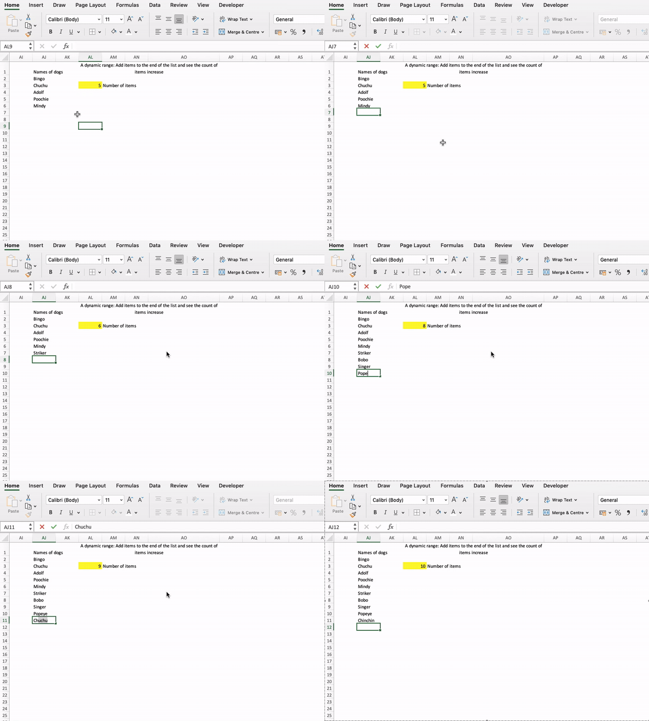
Want to see how to create a list that updates automatically when you add a new item to it?

These kinds of lists are called dynamic ranges. Dynamic ranges can be used to automatically generate the sums, total counts, averages, maximum and minimum values of a list you are updating in real time. We will use a tear-down tutorial to demonstrate how to set up dynamic ranges in MS Excel.

By stepping into the cell with the value that was updating the range count, we observe the name of the range is titled myDynamicRange. We can also see that a =COUNTA() function is wrapped around the range’s name, ensuring that only cells that are not blank are included in the count computation. We will now explore how myDynamicRange was set up, by going to the Name Manager (Formula >> Name Manager, or keyboard shortcut Ctrl+F3 in Windows).

The Name Manager dialog box shows the name of the range, and the range of cells the range name applies to. Unlike regular named ranges (read about this here) that simply reflect a cell reference (e.g. $C$3) or a range reference (e.g. $A$1:$A$1001), dynamic named ranges reflect a combination of cell references and 2 functions: =OFFSET() and =COUNTA(). We have discussed the function of =COUNTA() – it is a variant of the =COUNT() function that specifically counts non-blank cells in a range. We will spend some time understanding the =OFFSET function.

The =OFFSET() function is the key function for defining dynamic ranges. You can create any kind of range from any part of the worksheet, and with the OFFSET function syntax, you only need to define 5 attributes:

• the starting cell or base cell (Reference);
• the number of rows away from the starting cell your range will start from (Rows);
• the number of columns away from the starting cell your range will start from (Columns);
• the number of rows of your range (Height); and
• the number of columns of your range (Width)

The last two are optional – if they are left blank the function defaults them to 1.

Let’s break down the =OFFSET formula above to understand it in detail:

Reference = Demo!$AJ$1. This is the first item in the column. In our example, it is the title of the list.

Rows = 1. This is because we want the dynamic range to start 1 row after the reference, because we do not want the title of the list (“Names of dogs”) to be counted in the list. If you have a list that requires the title to also be counted, you can make this 0. This value can be a negative value, which will mean the range will start rows above the reference, instead of below.

Columns = 0. This is because we want the dynamic range to start on the same column of the reference. This can be a negative value, which means the range will start to the left of the reference, instead of to the right.

Height = COUNTA(Demo!$AJ:$AJ). Demo!$AJ:$AJ refers to all the cells in Column AJ on the sheet titled ‘Demo (our worksheet for this example). The COUNTA function counts the number of cells in the whole of column AJ that are not blank, with the assumption that they are on the list. The list of non-blank cells forms the number of rows in the dynamic range.

Width = 1. This is because we want a single column range. If we wanted a range cutting across 2 or more columns, this number can be changed to match this.

And this is how your dynamic range is set up in MS Excel.

• Two things about dynamic ranges:

• You have to dedicate an entire column to the dynamic range alone. If any other list is created below the dynamic range, the dynamic range counter will include it in the count.
• Dynamic ranges do not show up in the Name Box (box beside the formula bar) dropdown. To see the dynamic ranges in a workbook, you have to access the Name Manager.