Here’s a hack I uncovered while creating a mileage chart in MS Excel…

I was searching for mileage information (distance between cities) for 16 Nigerian cities online, and came across a mileage chart sheet. On downloading the sheet, turns out it had mileage information for 453 cities in total.

This was great, of course, as it had the information I needed. However, querying the table to get the specific information I required meant I had to filter to each of the 16 cities, scroll to the right to search for a corresponding city, and extract the mileage information manually to my mileage chart several times.

A mileage chart with 16 cities would need 256 data points (16 * 16). That sounded like a whole lot of work! So I experimented a bit and found a formula that gets the job done, easily!

This formula is set up so that you only have to create it once, and then you can drag it down and to the right and it fetches the data seamlessly. It’s that good!

So, what’s this magic formula? Here it is below:

=VLOOKUP($B4,[453citiestable],MATCH(C$3,[453citiesheaders],0),FALSE)

This formula is driven by the functionality of 2 key Excel features:

• Two Excel functions (=VLOOKUP and =MATCH)
• Cell references (mixed and absolute)

I’ll run a tear-down analysis to explain what each element does in detail below:

The =VLOOKUP function. Because this is essentially a table query, this function helps to return the value of a cell in a table given the corresponding item in the first row (the name of the city on the row axis – $B4 in the formula above), the entire table range (Kilometers! $A$1:$QK$453), and the number of the column it is on. We want this column number in the =VLOOKUP function to be dynamic and change as we move to a new column, so the =MATCH function does this job.

The =MATCH function. This function returns the position of any item on a list relative to the other items. If we listed the letters of the alphabet in the right order in a range and searched for the position of C using the =MATCH function, we would get the value 3 in return. The =MATCH function takes 3 arguments: the item we want to find (C$3 in the formula above), the range of the list (must always be either in single column or row, Kilometers!$A$1:$QK$1 in the formula above), and the specificity of the return (0 for exact match).

Cell references. This formula uses the appropriate cell reference to ensure the source magic formula is set up one time and will bring the right result, whether it is dragged to the right or downwards. The reference to the cities in the row header and column headers are mixed – for the row headers, the column is locked ($B4) so that the formula always references the starting column, and for the column headers, the row is locked (C$3) so that the formula always references the starting row. Check out this post for more on cell references.

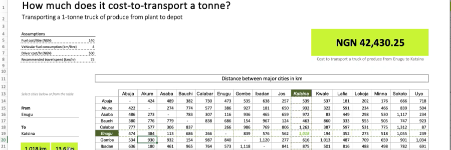
Want to see how I used this formula to create the feature image (“How much does it cost to transport a tonne…”) on this post? Check out my YouTube tutorial on 101 Excel Hacks (it is in 2 parts):

The final model I built – the cost-to-transport model – is available for free download here