Excel Hack 28: Use macros to put formulas in cells
To place a formula in a cell using Excel VBA, use the following code: Sub VBAFormula() Range(“A3”).Value = “=AVERAGE(A1:A2)” End Sub
To place a formula in a cell using Excel VBA, use the following code: Sub VBAFormula() Range(“A3”).Value = “=AVERAGE(A1:A2)” End Sub
=VLOOKUP() formulas typically force users to convert all their knowledge of a reference table into numbers. We know a table contains columns with clear headers such as ID, First Name, Last Name, Address, etc. And the =VLOOKUP function requires us to convert that column to a number (First Name on column B to column index
Ever encountered challenges in identifying the required column while using =VLOOKUP() on large, complex tables that stretch into several columns? There is an easy way out. Most users hard-code the column number in the VLOOKUP formula e.g. =VLOOKUP (“Bat Roger”,$B$4:$Y$83,16,FALSE). However, this number can be replaced with a =COLUMN() formula that will seek out the 16th
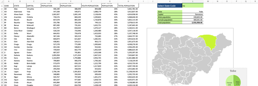
If you want to represent research or analysis based on geography, the preferred graphic is usually a map. Each geographic unit (continent, country or county) can be uniquely colored based an agreed color scale to represent the information to be communicated for that unit. When working with data spread over a diverse scale, having to manually

[One-line post alert] To do the above, use the formula below: =countif(cell reference of list B, cell reference of list A item)