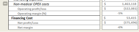
This hack shows how to insert a macro that provides users with a functionality to show and hide rows (or columns) in an Excel document. This feature can be used to bring an interactive dashboard feel to an Excel document, such as expanding and collapsing the component rows that make up a line item without using the native Excel group-ungroup feature, or to show instructions for using the rest of the dashboard in the first column and hide when not required.

This feature is added on using macros. There are two subs: A “hide row” and an “unhide row”, and both macros are attached to plus and minus miniature icons and activated by clicking them. The icons can be layered on top of one another to give an impression of a toggle function.

The code below hides rows 31 to 35, makes the minus sign (Picture 61) invisible and the plus sign (Picture 62) visible.

 Sub HideRows()

Rows(“31:35”).EntireRow.Hidden = False
ActiveSheet.Shapes.Range(Array(“Picture 61”)).Visible = msoFalse
ActiveSheet.Shapes.Range(Array(“Picture 62”)).Visible = msoTrue

End Sub

The code below makes rows 31 to 35 visible, makes the minus sign (Picture 61) visible and the plus sign (Picture 62) invisible.

Sub UnhideRows()

Rows(“31:35”).EntireRow.Hidden = False
ActiveSheet.Shapes.Range(Array(“Picture 61”)).Visible = msoTrue
ActiveSheet.Shapes.Range(Array(“Picture 62”)).Visible = msoFalse

End Sub

Once the icons are in place, the “Move but don’t size with cells” setting should be enabled in Picture Properties (click on the shape button and press Ctrl+1 to edit property).