Typically, when the =RANK() function is run in Excel it assigns a rank number to every item on the list in either ascending or descending fashion and will duplicate ranks where items are duplicated. However, sometimes you may have scenarios in which you need Excel to return a unique, un-duplicated rank for each item. For example, a business sales report that would feature the top 3 sales reps based on volume sales.

Let’s assume we have the dataset below as our starting point – a list of sales reps and their volume sales:

To rank these items based on the sales volume, we would apply a =RANK() formula in cell A3 to return the rank of the sales volume in C3 relative to the entire list ($C$3:$C$10), and drag this down till A10:

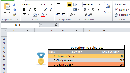
We could then return the name and sales volume of the top 3 reps in a performance league table on the report sheet by running a =VLOOKUP() formula on the rank number:

However, when we try to extend this =VLOOKUP() formula to the other numbers (2 and 3), we would encounter a #N/A error on number 3. This is because there is no rank 3 on the original ranking of the dataset; 2 sales reps recorded volume of 384 and thus were both allocated the 2nd rank.

To prevent this from happening, the formula below could be applied to rank the original dataset instead of the simple =RANK(C3,$C$3:$C$10,0) that was originally used:

=RANK(C3,$C$3:$C$10,0)+COUNTIF($C$2:C2,C3)

This formula basically does an initial ranking, then looks for the number of times that that sales volume has appeared in the list previously and adds this to the rank. The $C$2 is an absolute reference that locks the beginning of the list, while the C2 is a relative reference that moves as the formula is dragged to indicate the most previous reference on the list. In between these two references we are able to have a range that shows all the items on the list right before the one being evaluated in the formula. When we apply this the original dataset becomes:

And the performance league table now looks like this: